

unbalanced FORCES LAb
9/23/21
This is the Unbalanced Forces lab, a lab where we changed the weights on either side of a cart or a hanger and measured the change of acceleration using a motion sensor.
Overview
Research Question: 1. How does the net force of the cart affect its acceleration? 2. How does the total mass of a system affect its acceleration?
Experiment 1:
Independent Variable: the net force acting upon the cart
Dependent Variable: the acceleration of the cart
Control Variable: total mass of the hanger cart system, the hanger, and the track upon which the cart travels
The Controlled Variables
To keep the experiment controlled, we keep the total mass constant because an increase in mass would directly lead to an increase in inertia. We change the net force by moving weights between the hanger and the cart, keeping the total mass constant.
Experiment 2:
Independent Variable: the total mass of the system
Dependent Variable: the acceleration of the cart
Control Variable: the net force acting upon the cart, the hanger, and the track upon which the cart travels
The Controlled Variables
To keep the experiment controlled, we keep the net force the same to isolate that the only variable contributing to the change in acceleration would be the change in mass of the cart.
Collection of Data
To collect our data, we used a Motion Sensor to give us real time graphs of the movement and acceleration of the cart for both experiments.
Meet The Team


Procedure
Experiment 1:
- We positioned the cart at the end of the ramp and held on to it.
- We started the motion sensor.
- Then we let go of the cart and let it slide down the ramp.
- We stopped the cart with both hands before the hanger hit the ground.
- Record the total mass of the hanger (or net force)
- We then went into logger pro, and selected the portion of the velocity time graph generated by the motion sensor from when the cart begins to accelerate to when the cart stops. we pressed"linear fit" and collect the linear coefficient (the acceleration of the cart).
- Repeat the previous steps for different masses on the hanger. Remember to keep the total mass constant.
Experiment 2:
- We position the cart at the end of the ramp and hold on to it.
- We started the motion sensor.
- We let go of the cart and let it slide down the ramp.
- We stopped the cart with both hands before the hanger hit the ground.
- We recorded the mass of the cart.
- We then went into logger pro, and selected the portion of the velocity time graph generated by the motion sensor from when the cart begins to accelerate to when the cart stops. Press "linear fit" and collect the linear coefficient (the acceleration of the cart).
- Repeat the previous steps for different masses on the cart. The total mass of the system changes but the mass on the hanger should be constant.
Lab Setup
![20211025_091814[778].jpg](https://static.wixstatic.com/media/043c54_ff728d22315f46b8a165176b77036c54~mv2.jpg/v1/fill/w_600,h_340,al_c,q_80,usm_0.66_1.00_0.01,enc_avif,quality_auto/20211025_091814%5B778%5D.jpg)
Weights
Cart
Pulley
Hanger
Motion Sensor
Ramp
String
Raw Data
Experiment 1


Experiment 2

Better quality CSV files containing all raw data is also embedded below (first one is exp 1, second is exp 2)
Processed Data
Though some part of the processed data was already shown in the raw data section, the explanations of how we calculated these data figures will be explained here.
Experiment 1
We first started our calculations by determining the acceleration from the velocity time graph made from the motion sensor graph shown in the raw data above, with constant mass of 1.675 kg. The net force acting upon the cart is a tension force generated by the force of gravity (Fg) on the hanger. this can be calculated using the formula Fg = mg, where m is mass and g is the acceleration of gravity, in this case, g = 9.8.
Using this information, we were able to create the graph below.

The graph above shows how the net force upon the car affects the acceleration f the cart directly. When the car has a net force of zero acting upon it, its acceleration would therefore be zero. This is why the best model for this set of data would be the proportional model over that of the linear model, as it captures the idea that at zero net force, the acceleration would be at constant zero too. The equation for this model is 1.4762*∑F, where the slope of the graph/ the constant acceleration is 1.4762 m/s^2, meaning for every newton in force, the acceleration increases by 1.4762 m/s^2.
Experiment 2
We processed the data of this experiment by, again, calculating the acceleration from the velocity time graphs derived from the motion sensor in logger pro. In this case, we kept the mass of the hanger constant at 0.05 kg, as well as a constant net force of 0.49 newtons, which was calculated, again, using the formula of Fg = mg.
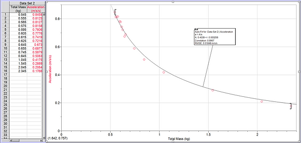
From the results of Experiment 2, we were able to create the graph shown above, which shows how the mass of a system affects the acceleration of the objects inside of the system. There were two models presented as possible candidates for this data set: quadratic and inverse. The reason why our group went with the inverse fit was because when the quadratic model crosses zero, it would not make sense as there is nothing to accelerate with no mass. The inverse fit, however, gets infinity close but never approaches zero, therefore still staying inside the realm of possibility. The equation for this model is Acceleration = 0.454/mass. The inverse model does not have a constant slope but as the total mass of the system increases, the acceleration decreases by less and less.
Downloads of the two graphs are linked below
Processed Data
Conclusion
These two labs helped us to prove Newton's Second Law of motion that Net Force = Mass * Acceleration. From our graphs, we conclude that the acceleration of an object iis directly correlated to the Net Force (∑F) acting on upon the object and the Mass of the object. This is supported by our experiments as the predictions offered by our models closley resemble real life results. In Experiment 1, the proportional model shows that Acceleration = A * ∑F, we can see that A = 1/mass, which was estimated to be (), the estimate made by the graph, is close to the actual value of 1/0.675. In Experiment 2, the inverse model shows that Acceleration = B/mass, we can see that the net force B was estimated by the model to be (), and is close to the actual value of 0.49N. Our results show that: as the force acting upon an object increases, the acceleration of the object also increases, and as the mass of an object increases, the acceleration of the object in turn decreases. This makes sense as a heavier object is harder to move/accelerate than a lighter one. Therefore, these experiments heed us to prove Newtons 2nd Law of Motion,
F = ma
Newton's Second Law is everywhere. It connects Force to Mass and Acceleration which can be used to describe all types of motion in our lives everday.
Conclusion
Uncertainties and Limitations
Experiment 1
Uncertainty in this experiment was the range of the data. Due to the limitation that we could not have the cart accelerating too fast as it might cause some damages to the cart, we did not have large net forces acting on the cart. Another uncertainty was the exclusion air resistance as the force applied on the car. The friction of the tracks (which was minimal) also plays a role in the force applied on the cart, both these forces are negligible due to their minimal contributions for the purposes of the lab.
Experiment 2
Some error in the collection of the data might be apparent, the two experiments have roughly the same uncertainties regarding not collecting enough data to be confident enough.
Improvements?
For both experiments, one way to improve the investigation is to collect a larger range of data. It is always beneficial to have a bigger collection of data so we can fit the model much accurately.